User guide

Introduction

Nearest neighbor search is the problem of finding the closest data points to a given query point in a multi-dimensional space, commonly used in recommendation systems, image retrieval, and machine learning. A brute-force approach involves computing the distance between the query and every data point in the dataset, which guarantees exact results but becomes computationally infeasible as the dataset grows, especially in high-dimensional spaces where the cost is O(Nd) (with N being the number of points and d the dimensionality).

To overcome this, approximate nearest neighbor (ANN) search techniques trade off some accuracy for significant speed improvements. One of the most efficient ANN methods is Hierarchical Navigable Small World (HNSW), which organizes data into a multi-layered small-world graph, enabling fast traversal with logarithmic search complexity. HNSW efficiently balances speed and accuracy, making it a popular choice for large-scale nearest neighbor search problems.

One of the main drawbacks of the HNSW algorithm is its high memory consumption. Unlike tree-based or hash-based methods, HNSW stores a graph where each node (data point) maintains multiple bidirectional connections, leading to significant memory overhead, especially for large datasets. Additionally, due to its graph-based nature, HNSW is inherently not designed for distributed execution, as the graph structure requires global connectivity for efficient search traversal. This makes it challenging to partition the graph across multiple machines without degrading performance. However, sharding can be used to distribute HNSW by splitting the dataset into multiple independent indices, each residing on a different machine. Queries can then be routed to relevant shards based on techniques like geometric partitioning or clustering, and the results can be merged to approximate a global nearest neighbor search.

While this approach introduces trade-offs, such as potential cross-shard communication and slightly lower recall, it enables scaling HNSW to massive datasets that cannot fit into a single machine’s memory.

Hnswlib spark is an implementation of this idea built on top of Apache Spark.

Indexing

Apache Spark operates in a master-worker model where the driver program orchestrates execution, manages the DAG (Directed Acyclic Graph) of tasks, and coordinates data shuffling between stages.

The driver communicates with executors, which are distributed across a cluster and handle task execution.

Each executor is a JVM process running on a worker node, allocated multiple task slots, where each slot represents a unit of parallelism. Traditionally, a task in Spark runs within a single task slot, utilizing one CPU core, meaning that if an executor has four cores, it can run up to four tasks in parallel, assuming four slots are allocated.

However, with stage-level scheduling, Spark introduced the flexibility to assign multiple CPU cores to a single task, changing the traditional execution model.

This is particularly useful for building distributed HNSW indexes, as the indexing process is highly multithreaded, and this allows us to create a small number of large indices rather than many fragmented ones.

Creating a distributed knn index with hnsw spark is easy and can be accomplished within a few lines.

Avoid using ephemeral resources like AWS spot instances for executors. Since indices reside in memory, losing an executor means they cannot be recovered.

• python
• scala

• from pyspark_hnsw.knn import HnswSimilarity
  
  hnsw = HnswSimilarity(
      identifierCol='id',
      featuresCol='features',
      distanceFunction='cosine',
      numPartitions=2,
      numThreads=2,
      k=10,
      m=16,
      efConstruction=200,
      ef=10,
  )
  
  model = hnsw.fit(items)
  

• import com.github.jelmerk.spark.knn.hnsw.HnswSimilarity
  
  val hnsw = new HnswSimilarity()
    .setIdentifierCol("id")
    .setFeaturesCol("features")
    .setDistanceFunction("cosine")
    .setNumPartitions(2)
    .setNumThreads(2)
    .setK(10)
    .setM(16)
    .setEfConstruction(200)
    .setEf(10)
  
  val model = hnsw.fit(items)
  

The input DataFrame (e.g., items) must contain two columns:

• id - can be a long, int or string

• features - can be a vector, sparse vector, float array or double array

• distanceFunction - one of bray-curtis, canberra, cosine, correlation, euclidean, inner-product, manhattan

• numPartitions Sets the number of shards to create. Fewer partitions are generally better, as more partitions speed up indexing but can significantly slow down queries unless the data is pre-partitioned.

• numThreads Controls the number of CPU cores used for indexing a shard and cannot exceed the cores available on an executor. It’s best to set this value equal to the executor’s core count for optimal performance.

• k Sets the number of similar matches to return

• m The maximum number of bi-directional connections (neighbors) per node. Higher values improve recall but increase memory usage and search time.

• ef The size of the dynamic candidate list during the search. A higher ef improves recall at the cost of search speed.

• efConstruction Similar to ef, but used during index construction. A higher efConstruction results in a more accurate graph with better recall but increases indexing time and memory usage

After fitting the model, the Spark UI will show running tasks even after the fit method returns.

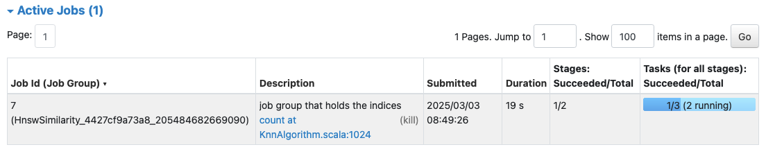
Each task reserves 2 cores (as set by numThreads) and retains cluster resources until the model is explicitly released by calling dispose() on the model.

Each task starts a gRPC service for querying the index and registers itself with the driver once the service is running. The fit method completes when all partitions are registered, but the tasks continue running in the background.

Querying

To query the index you call transform on the produced model.

• python
• scala

• model.transform(queries)
  

• model.transform(queries)
  

The query DataFrame (e.g., queries) must contain one column:

• features - must match the type and dimensionality of the features column in the input DataFrame

The output dataframe produced by transform will include an additional column, prediction by default. It contains an array of up to k structs, each with a neighbor and distance field. Neighbor is the identifier of the item matched, the distance indicates how far the item is removed from the query Smaller distances indicate that the index item is closer to the query.

The prediction is obtained by querying all shards through their gRPC APIs for the top k items and selecting the closest k items from the combined result list.

Pre-partitioning

Querying many shards can be expensive. To optimize, co-locate nearby items in the same index and skip irrelevant shards during querying. Use a partitioning algorithm to assign each item a partition, represented as an integer column in the input dataset (partition in the example).

The queries DataFrame should include a column with an array of partitions to query (partitions in the example).

Ensure custom partitions are balanced, with roughly equal sizes.

• python
• scala

• from pyspark_hnsw.knn import HnswSimilarity
  
  hnsw = HnswSimilarity(
      identifierCol='id',
      featuresCol='features',
      partitionCol='partition', # column that contains the partition index items will be assigned to
      queryPartitionsCol='partitions', # column that contains the partitions that will be queried for a query
      numPartitions=2,
      numThreads=2,
  )
  
  model = hnsw.fit(items)
  

• import com.github.jelmerk.spark.knn.hnsw.HnswSimilarity
  
  val hnsw = new HnswSimilarity()
    .setIdentifierCol("id")
    .setFeaturesCol("features")
    .setPartitionCol("partitions") // column that contains the partition index items will be assigned to 
    .setQueryPartitionsCol("partitions") // column that contains the partitions that will be queried for a query
    .setNumPartitions(2)
    .setNumThreads(2)
    
  
  val model = hnsw.fit(items)
  

Replicating indices

More shards speed up indexing but often slow down querying since each shard must be searched. To improve query speed, use index replicas. Adding a single replica doubles the query capacity per shard

To add query replicas, set the numReplicas parameter on the model.

• python
• scala

• from pyspark_hnsw.knn import HnswSimilarity
  
  hnsw = HnswSimilarity(
      identifierCol='id',
      featuresCol='features',
      numPartitions=2,
      numReplicas=1, # configure 1 replica
      numThreads=2,
  )
  
  model = hnsw.fit(items)
  

• import com.github.jelmerk.spark.knn.hnsw.HnswSimilarity
  
  val hnsw = new HnswSimilarity()
    .setIdentifierCol("id")
    .setFeaturesCol("features")
    .setNumPartitions(2)
    .setNumReplicas(2) // configure 1 replica
    .setNumThreads(2)
    
  
  val model = hnsw.fit(items)
  

Saving and loading the model

It is possible to save and load an index.

• python
• scala

• from pyspark_hnsw.knn import HnswSimilarityModel
  
  model.write().overwrite().save(path)
  
  loaded = HnswSimilarityModel.read().load(path)
  

• import com.github.jelmerk.spark.knn.hnsw.HnswSimilarityModel
  
  model.write.overwrite().save(path)
  
  val loaded = HnswSimilarityModel.read.load(path)
  
  

Appending to an existing index

To append to an index, first save it, then reference the output path when creating a new model. The types of the input dataframe must match that of the initial model. The number of partitions must match that of the initial model

To append to an index, save it first, then use the output path when creating a new model. The input dataframe’s types must match the types used to construct the initial model.

It is not possible to change the partition count when appending to an existing index.

Indices are limited by executor memory. When appending to an index, ensure ample memory headroom. You may want to over partition to avoid exceeding memory limits in the future.

• python
• scala

• from pyspark_hnsw.knn import HnswSimilarity
  
  items = spark.table("items") # Must match the data types of the initial model
  
  hnsw = HnswSimilarity(
      identifierCol='id',
      featuresCol='features',
      numPartitions=2,
      numThreads=2, # Must match the number of partitions in the initial model
      initialModelPath=path, # Location where your model is saved.
  )
  
  model = hnsw.fit(items)
  

• import com.github.jelmerk.spark.knn.hnsw.HnswSimilarity
  
  val items = spark.table("items") // Must match the data types of the initial model
  
  val hnsw = new HnswSimilarity()
    .setIdentifierCol("id")
    .setFeaturesCol("features")
    .setNumPartitions(2) // Must match the number of partitions in the initial model
    .setNumThreads(2)
    .setInitialModelPath(path) // Location where your model is saved.
    
  
  val model = hnsw.fit(items)
  

Evaluating index accuracy

Approximate nearest neighbor (ANN) search sacrifices some accuracy for much faster queries.

Hnswlib Spark includes a brute-force nearest neighbor search implementation, which is slow but always accurate. You can use it in conjunction with KnnSimilarityEvaluator to evaluate the quality of the results from the HNSW index.

Brute-force knn search is very slow, so use a small sample to assess accuracy.

• python
• scala

• from pyspark.ml import Pipeline
  
  from pyspark_hnsw.evaluation import KnnSimilarityEvaluator
  from pyspark_hnsw.knn import BruteForceSimilarity, HnswSimilarity
  
  hnsw = HnswSimilarity(
      identifierCol='id',
      featuresCol='features',
      numPartitions=1,
      numThreads=2,
      k=10,
      distanceFunction='cosine',
      predictionCol='approximate' # the approximate predictions will be stored in this column
  )
  
  bruteForce = BruteForceSimilarity(
      identifierCol=hnsw.getIdentifierCol(),
      featuresCol=hnsw.getFeaturesCol(),
      numPartitions=1,
      numThreads=2,
      k=hnsw.getK(),
      distanceFunction=hnsw.getDistanceFunction(),
      predictionCol='exact', # the exact predictions will be stored in this column
  )
  
  pipeline = Pipeline(stages=[hnsw, bruteForce])
  
  model = pipeline.fit(items)
  
  output = model.transform(queries)
  
  evaluator = KnnSimilarityEvaluator(approximateNeighborsCol='approximate', exactNeighborsCol='exact')
  
  accuracy = evaluator.evaluate(output)
  
  print(f"Accuracy: {accuracy}")
  

• import org.apache.spark.ml.Pipeline
  
  import com.github.jelmerk.spark.knn.bruteforce.BruteForceSimilarity
  import com.github.jelmerk.spark.knn.evaluation.KnnSimilarityEvaluator
  import com.github.jelmerk.spark.knn.hnsw.HnswSimilarity
  
  val hnsw = new HnswSimilarity()
    .setIdentifierCol("id")
    .setFeaturesCol("features")
    .setNumPartitions(1)
    .setNumThreads(2)
    .setK(10)
    .setDistanceFunction("cosine")
    .setPredictionCol("approximate") // the approximate predictions will be stored in this column
  
  val bruteForce = new BruteForceSimilarity()
    .setIdentifierCol(hnsw.getIdentifierCol)
    .setFeaturesCol(hnsw.getFeaturesCol)
    .setNumPartitions(1)
    .setNumThreads(2)
    .setK(hnsw.getK)
    .setDistanceFunction(hnsw.getDistanceFunction)
    .setPredictionCol("exact") // the exact predictions will be stored in this column
  
  val pipeline = new Pipeline()
    .setStages(Array(hnsw, bruteForce))
  
  val model = pipeline.fit(items)
  
  val output = model.transform(queries)
  
  val evaluator = new KnnSimilarityEvaluator()
    .setApproximateNeighborsCol("approximate")
    .setExactNeighborsCol("exact")
  
  val accuracy = evaluator.evaluate(output)
  
  println(s"Accuracy: $accuracy")
  

Converting vectors

Hnswlib Spark supports MLlib vectors, float arrays, and double arrays as features. MLlib vectors use the most memory, double arrays use less, and float arrays use the least but with lower precision, affecting accuracy. VectorConverter allows conversion between these types.

• python
• scala

• from pyspark_hnsw.conversion import VectorConverter
  
  converter = VectorConverter(inputCol="featuresAsMlLibVector", outputCol="features", outputType="array<float>")
  
  converter.transform(items)
  
  

• import com.github.jelmerk.spark.conversion.VectorConverter
  
  val converter = new VectorConverter()
    .setInputCol("featuresAsMlLibVector")
    .setOutputCol("features")
    .setOutputType("array<float>")
  
  converter.transform(items)
  

outputType must be one of array<float>, array<double> or vector

Normalizing vectors

By normalizing vectors to unit length, inner product search can be used to achieve the same results as cosine distance since the cosine similarity between two normalized vectors is directly proportional to their inner product. This approach avoids the computational overhead of explicitly computing cosine distances, making queries faster and more efficient.

• python
• scala

• from pyspark_hnsw.linalg import Normalizer
  
  normalizer = Normalizer(inputCol="vector", outputCol="normalized_vector")
  
  normalizer.transform(items)
  
  

• import com.github.jelmerk.spark.linalg.Normalizer
  
  val normalizer = new Normalizer()
    .setInputCol("features")
    .setOutputCol("normalizedFeatures")
  
  converter.transform(items)